I’ve always been fascinated with advanced analytics in sports. Leveraging the mountains of data that are collected to unlock new perspectives and influence decision-making has heavily shaped every sport in the last few decades. While advanced analytics is no silver bullet, it plays a very important role in the decision-making process and should always be considered when evaluating options. This fascination has naturally led to curiosity about metrics such as SP+, ESPN’s FPI, the Expected-Points-Added statistic — basically any interesting metric I’ve come across.
Subsequently, this interest led to me developing my own rudimentary models to predict college football single-game outcomes. I developed two models, both using logistic regression, trained on single-game regular season data pulled from the last four seasons (Fall 2021 – Fall 2024). At a high level, model A is the base model, using nearly every variable in the dataset as a predictor. Model B is the slimmed model, which used an algorithm to remove insignificant predictors — leaving just 12. There isn’t necessarily an advantage to either method, though models with fewer predictors tend to be less prone to overfitting.
After testing, both models were able to predict game outcomes with an accuracy over 75%:
| Base Model | 78.53% |
| Slimmed Model | 77.84% |
Information on how these accuracies were calculated can found in the section below.
Methodology
If you’re more interested in my findings than the technical aspects, continue to the next section.
This model was built using the logistic regression machine learning algorithm in RStudio, with heavy usage of the rsample package for training/testing data splits. Other packages I used frequently are cfbfastR and dplyr.
Regarding cfbfastR, this package has been extremely helpful and makes it easy to scrape tons of up-to-date college football data. Carrying out this passion project would not have been possible without it and I highly, highly recommend it to anybody looking to get into sports analytics. Using cfbfastR, I was able to scrape all regular season games between FBS schools1 from 2021 to 2024. This contained single-game information; things like the box score, team statistics, crowd size, and so on. Additionally, I filtered out neutral site games, as I wanted to keep the data as uniform as possible.2
As of October 9th, 2025, the Neutral Site Model has been created and can be read about here.
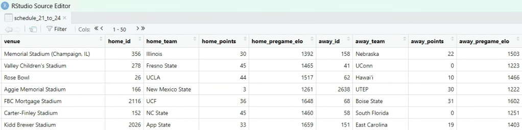
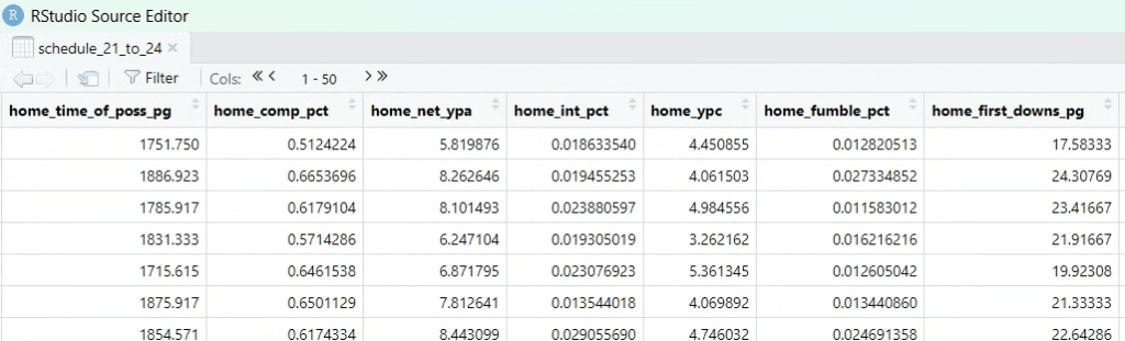
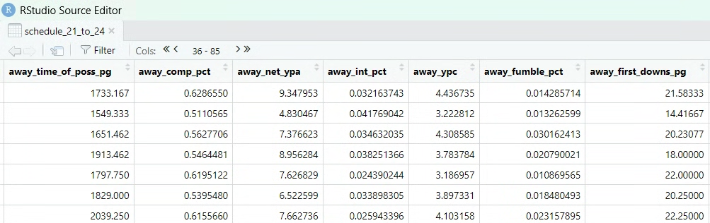
Next, I scraped all of the season statistics3 for each school and performed a left join on the data frame containing regular season games. Determining the structure for this combined data frame took a lot of thinking and researching different methods, but I ultimately decided on having both home team and away team statistics within one row. These were designated accordingly:
After some cleaning and calculation of specific statistics I wanted to include4, I started to build the model. The first step involved splitting the data into a training set and a testing set. This allowed me to gauge how accurate the models will be when working with unseen data.
In my first model, I included 43 predictors (variables) — nearly every single metric in the combined data frame. I actually included all ~60 of them to start, but received a warning message that “fitted probabilities numerically 0 or 1 occurred”, suggesting multicollinearity or overfitting (or both). I removed predictors that had extremely low p-values; things like home/away offensive plays per game, drives per game, yards per kick return, and so on. That left me with the 43-variable model that I used as my “total” or “base” model.
After blueprinting the base model, I trained it on the training set to determine predictor coefficients and overall accuracy — which will be discussed in the following section.
From there, I decided to run a stepwise regression to slim down the model. While it was good to have a base model to work with, I wanted to see if I could remove predictors in order to increase accuracy, along with potentially decreasing overfitting. For those unfamiliar with stepwise regression, it essentially removes predictors that are determined insignificant through an algorithm.5 The subsequent stepwise model contained 12 predictors. If you’re uninterested in my ramblings on the nuances of stepwise regression, skip the next two paragraphs:
It is important to note that the final stepwise regression model (the model that will be used for upcoming season, not the model that was used to estimate accuracy), trained on the entire dataset (as opposed to being trained on a training/testing split), was slimmed down to 11 predictors. While it should perform similarly to the stepwise regression model that had 12 predictors, it is difficult for me to say with absolute certainty.
The reason that the stepwise model used for estimating accuracy and the final stepwise model have a different number of variables is that the stepwise regression function removes non-essential predictors based on the data that the model is trained on. I only created the first stepwise model as a means of gauging accuracy — it’s not the final model that will be used to predict upcoming games.6
Additionally, I want to note that the stepwise regression was done in both directions, not solely forward or backward.
Concerning the models that will be used throughout the upcoming season, I considered adding 2025 games to the training data at the conclusion of each week. However, I decided against this, as I didn’t want to be constantly retraining and jeopardizing having consistent predictors for the stepwise model.
As for calculating accuracy, I wrote utilized a for loop that performed the following actions 10,000 times, for both the base model and slimmed stepwise model:
- Split the master data frame (containing all games from 2021 to 2024) into testing and training data sets
- Created a new data frame for both training and testing data sets, in both of which I:
- Created a new column named “predicted_win_probability” that ran the model and recorded the home team’s win probability
- Created a new column named “predicted_win” that utilized an if-else statement to determine if the model had predicted a win or loss for the home team. This column was a binary 0/1
- Calculated training and testing accuracy by recording the percentage of matches in columns “predicted_win” and “home_result”. These percentages were assigned to variables train_accuracy and test_accuracy
- Added the iteration, train_accuracy, and test_accuracy values into a previously created data frame using rbind()
For an example of one of the loops I wrote, see below:
For Loop
iterations = 1000

accuracy_results_1 = data.frame(Iteration = numeric(),
                              Train_Accuracy = numeric(),
                              Test_Accuracy = numeric())

for (i in 1:iterations) {

  # performing split
  data_split = initial_split(schedule_21_to_24, prop = 0.8)
  model_training_loop = training(data_split)
  model_testing_loop = testing(data_split)

  # making predictions and adding into data frames
  train_predictions_loop = model_training_loop %>%
    mutate(predicted_win_probability = predict(total_model_1.0, newdata=., type = "response"))

  train_predictions_loop = train_predictions_loop %>%
    mutate(predicted_win = ifelse(predicted_win_probability >= 0.5, 1, 0))

  test_predictions_loop = model_testing_loop %>%
    mutate(predicted_win_probability = predict(total_model_1.0, newdata=., type = "response"))

  test_predictions_loop = test_predictions_loop %>%
    mutate(predicted_win = ifelse(predicted_win_probability >= 0.5, 1, 0))

  # calculating accuracy
  train_accuracy = mean(train_predictions_loop$predicted_win == train_predictions_loop$home_result) # calculates % of times the two columns match
  test_accuracy = mean(test_predictions_loop$predicted_win == test_predictions_loop$home_result)

  # adding into results df
  accuracy_results_1 = rbind(accuracy_results_1, data.frame(Iteration = i,                                                        Train_Accuracy = train_accuracy,                                                       Test_Accuracy = test_accuracy))
}
Extremely late in the process (just a handful of days before publishing), I realized I had forgotten a key step in this for loop: retraining the model with each iteration. I was effectively re-splitting the training and testing data repeatedly, without actually applying it to the model. As a result, the model would sometimes have lots of its training data overlap with the testing data, and vice versa. This caused a much wider range of accuracies than there would have been had I included the retraining step in the loop.
My goal, had I included this step, was to calculate the accuracy distribution across 10,000 training/testing data splits, with the model being retrained 10,000 times. This would have allowed me to hone in on a median accuracy that eliminated both very “lucky” and very “unlucky” splits that caused accuracy in a single instance of the model to skew one way or another.
As I wrote it, the for loop assesses how well the model, trained on a fixed set of data, holds up to different resamples. This is great for testing things like overfitting for this specific model and its training data. Unfortunately, not as relevant for this case as the previously described method would have been.
I spent quite some time considering whether or not I should redo these for loops to better fit my use-case. issue was that these for loops were written over three months ago. While I don’t believe this slight change in the for loop would compromise my work done after running it, I would still be forced to reevaluate dozens of hours of work.
Ultimately, I decided to leave it as is, given the purpose for the for loop was solely to get an estimate of how accurate both models would fare in a real-world context; a figure I will actually be able to calculate as the upcoming season plays out. Additionally, while the distribution of accuracies is certainly not reliable under this method — the range in accuracies is far inflated as previously mentioned — the median accuracy would have likely been the same, within 1-2%.
Constraints
The typical constraints that apply to any statistic model are present here. Football is a random game. Every season, game, drive, and play contains some inherent level of luck. The ball may bounce favorably for one team, the wind may blow in a certain direction, the officiating crew may make a certain call. While we like to see football as a game of absolutes (“You are what your record says you are.” – Bill Parcells), this is certainly not the case. Rather than seeing game outcomes as a binary statement that determines if Team A is better than Team B, I find it much more useful to think in terms of sample sizes and probabilities. Sure, Team A may have beaten Team B, but Team A only had a 30% chance of beating Team B at all (assume this is true for the sake of discussion). It just so happened that, due to random factors that include those outlined above, Team A happened to win this single game. We see this all the time in college football.
One of the most eye-opening statistics I’ve seen, a statistic which actually got me interested in advanced analytics, is Parker Fleming’s (@statsowar) weekly aggregation of Net Success Rates. After enduring a brutal watch for my Longhorns @ Texas Tech in 2022, I came away from the game feeling like we had won down-to-down, but we somehow still lost (largely thanks to Tech completing 6 of 8 fourth-down attempts). This tweet captured why it felt that way:
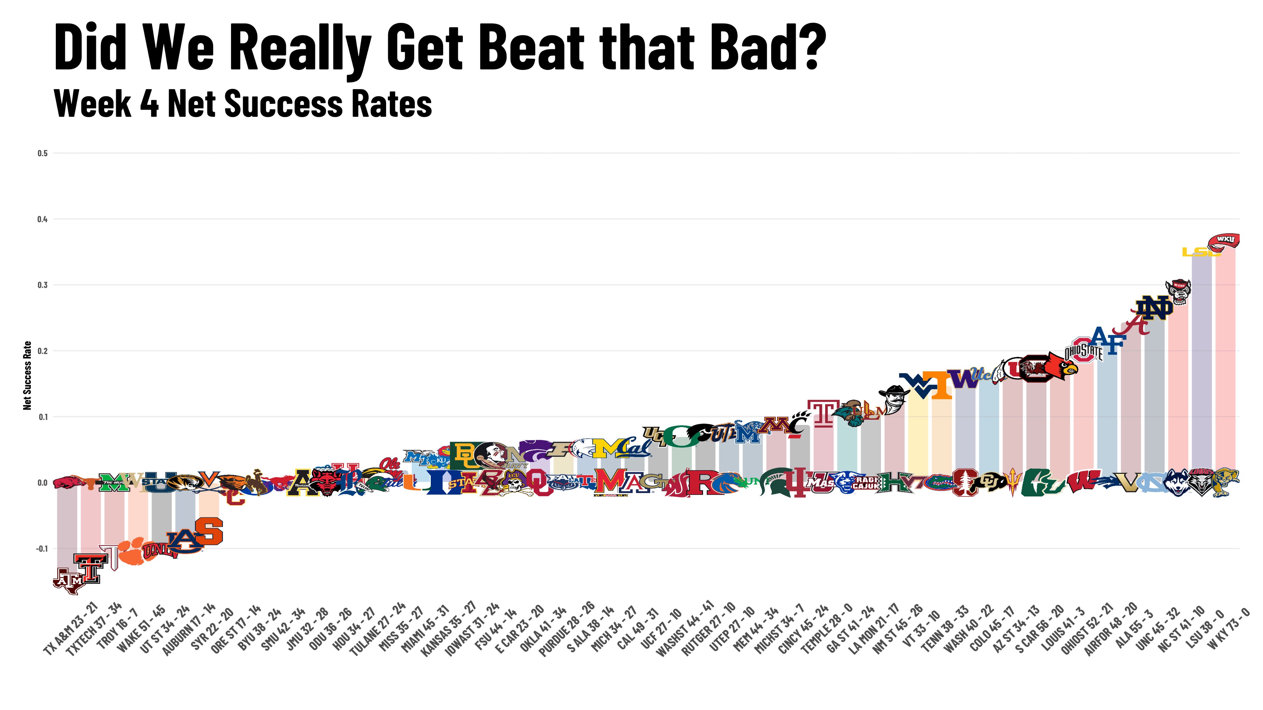
Texas Tech was less successful down-to-down, but a handful of plays shifted that game in their favor. This is not to say that their win was lucky by any means — it’s quite common in close football games to have only a few plays determine the outcome. Rather, it’s to emphasize this fact that only a handful of plays can influence a game, and therefore, a season. With any small sample size, randomness can be present, and that’s exactly what people who view sports through an analytical lens are talking about when referring to luck.
Further, this demonstrates that advanced analytics are only one tool in a vast toolkit with which you can evaluate football. No model will ever be able to accurately and consistently predict whether a player is hungover, whether the sun will hit a receiver’s eyes, and so on. Games are played as single instances, so the probabilities that any model produces don’t have the requisite sample size to properly bear out (if the probabilities are even accurate to begin with). Again, football is full of small sample sizes at multiple units of measurement (games per season, drives per game, fourth-down attempts, etc.), which contributes to the randomness and upsets that we all love the sport for.7
The constraint that is most specific to my model stems from the fact that the model was retroactively trained on an entire season’s worth of data. This means that when trying to predict a game in Week 2 of 2022, the model was provided the end of season statistics for both teams. This gave the model a much better chance of accurately predicting early season upsets, when in reality, as the season played out, it was clear that the “underdog” was actually a much higher quality team.
For example, in Week 3 of 2022, #25 Oregon (1-1) was hosting #12 BYU (2-0). Oregon beat BYU 41-20 and would go on to have a strong season (10-3), while BYU would have a decent, but not noteworthy season as a G5 independent (8-5). However, at the time, this was considered a close matchup, with Oregon only being favored by 3.5 points. Given that home-field advantage is often regarded as worth 3 points when calculating the spread, Vegas was essentially saying that Oregon was only 0.5 points better than BYU on a neutral field. Obviously, we saw this to be untrue as the season went on.
However, my slimmed model predicted a 96.1% probability that Oregon would win that game. This clearly runs counter to what Vegas thought at the time. This is because my model was given both teams’ season-end data, when it was clear that Oregon was the vastly superior team. Taking a step back, this means that my model’s preliminary accuracy rate is somewhat inflated at ~78%.
However, this shouldn’t be an issue moving forward, as games will be predicted in real-time, and season statistics will update week-to-week. However, this will inevitably result in a decrease in accuracy. Realistically, I hope for my model to sit around 67% accurate in predicting games as the upcoming season plays out.
Interesting Findings
Now that I’ve described my model and its intricacies, we can discuss the interesting stuff. Not only does the model predict a handful of upsets in the testing data, but it also provides perspective on some of the most unlikely upsets and what I’ve dubbed “nail-biter games”.8
It should be noted that the testing data only includes 573 games of the 2861 that occurred within the aforementioned criteria from 2021 to 2024, adhering to the 80/20 split between training and testing data. These were picked at random, so some notable games may not be present. It should also be noted that these findings come from the slimmed model, as opposed to the base model.
Upsets Predicted
I’ll start with upsets that my model predicted to occur. Again, these must be taken with a caveat, since these predictions didn’t occur in real-time, but only after the season concluded. I’ve decided to only include upsets that occurred in Week 8 or later in an attempt to mitigate this issue.
| Season, Week | Home Team | Away Team | Predicted Win Probability | Interesting Notes |
| 2021, Week 12 | #23 Utah (7-3): 38 | #3 Oregon (9-1): 7 | 82.7%, Utah | Utah converted 11/14 third downs |
| 2022, Week 13 | #21 Oregon State (8-3): 38 | #9 Oregon (9-2): 34 | 58.1%, Oregon State | Oregon State completed 6/13 passes for 60 yards and 2 INT; QBR of 10.4 |
| 2024, Week 11 | #16 Ole Miss (7-2): 28 | #3 Georgia (7-1): 10 | 62.8%, Ole Miss | Ole Miss outgained Georgia by 152 yards |
Having trouble viewing the table?
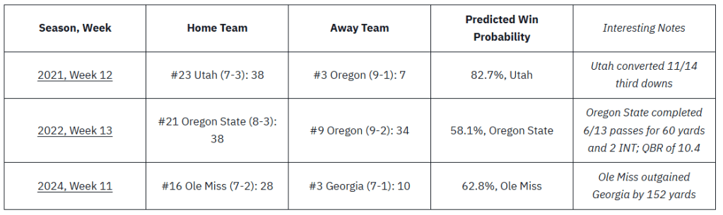
While it’s difficult to form any substantive conclusions about what these upsets have in common due to the small sample size (I can’t hammer this point enough), it is interesting that all of the underdogs won the turnover battle if you include turnovers on downs.9
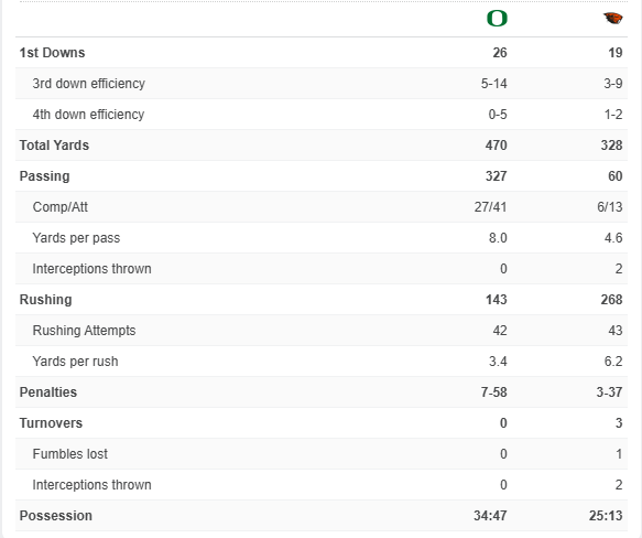
On a random note, while I couldn’t fit it all into the notes column, that Oregon State vs. Oregon game has one of the weirdest box scores I’ve ever seen. Oregon won in nearly every statistic, but the game was decided on fourth downs:
Biggest Upsets According to Model
Here are some of the biggest upsets from the model’s perspective; games that absolutely should not have had the outcome they did. These games were also only selected if they were in Week 8 or later of their respective seasons.
| Season, Week | Home Team | Away Team | Predicted Win Probability | Interesting Notes |
| 2021, Week 10 | TCU (3-5): 30 | #12 Baylor (7-1): 28 | 16.3%, TCU | TCU passed for 468 yards; Baylor only allowed >300 yards passing one other time all season |
| 2021, Week 11 | Texas (4-5): 56 | Kansas (1-8): 57 | 3.7%, Kansas | Kansas won the turnover battle 4-0 |
| 2024, Week 13 | Oklahoma (5-5): 24 | #7 Alabama (8-2): 3 | 19.5%, Oklahoma | Oklahoma had 68 passing yards |
Alternative Table View

There were a number of other upsets with win probabilities in 30-40% range, but I only included the extremes. Within the 573 game sample, there were very few instances where the model predicted an extremely low probability of a win (<5%), with the win actually occurring.
Again, it is interesting that the underdog won the turnover battle in each game — similar to the prior table. It’s very possible that this becomes a trend as the upcoming season plays out. However, the similarities between the games largely end there. For example, TCU outgained Baylor by over 150 yards, while Texas did the same to Kansas in a loss.
Biggest Nail-Biters
This is one of my favorite uses of the model. Since the model evaluates teams using their season-end statistics, we get a clear picture of the quality of each team. Regardless of when a game is played, we can determine if a team played up or down to its competition, based on the team’s quality (based on their entire body of work). Because of this, I’m able to evaluate games from all weeks of the season without compromising the results, not just after a certain week.
For reference, I define a “nail-biter” as a game in which a high quality team narrowly escapes an upset. More specifically, I used the criteria of the better team having a ≥ 80% chance of winning paired with a single-digit margin of victory.
| Season, Week | Home Team | Away Team | Predicted Win Probability | Interesting Notes |
| 2021, Week 2 | #8 Notre Dame (1-0): 32 | Toledo (1-0): 29 | 88.0%, Notre Dame | Toledo won the turnover battle 3-1 |
| 2022, Week 4 | #12 LSU (2-1): 34 | Arkansas (2-1): 31 | 90.7%, LSU | Arkansas possessed the ball for almost 9 more minutes than LSU |
| 2022, Week 4 | SMU (2-1): 34 | TCU (2-0): 42 | 90.0%, TCU | SMU went 4/4 on fourth-down attempts |
| 2022, Week 6 | #19 Kansas (5-0): 31 | #17 TCU (4-0): 38 | 80.0%, TCU | Kansas outgained TCU 540-452, but went 1/3 on fourth-down attempts |
| 2023, Week 10 | #7 Texas (7-1): 33 | #23 Kansas St (6-2): 30 | 80.8%, Texas | Both teams combined for 4/28 on third-down attempts |
| 2023, Week 13 | Auburn (6-5): 24 | #8 Alabama (10-1): 27 | 88.1%, Alabama | Auburn lost the turnover battle 3-0 and was outgained by 114 yards |
| 2024, Week 7 | #23 Illinois (4-1): 50 | Purdue (1-4): 49 | 94.9%, Illinois | Purdue almost doubled their season YPG (536) |
| 2024, Week 13 | Minnesota (6-4): 25 | #4 Penn State (9-1): 26 | 82.7%, Penn State | Minnesota possessed the ball for 34 minutes despite losing the turnover battle 2-0 |
Alternative Table View
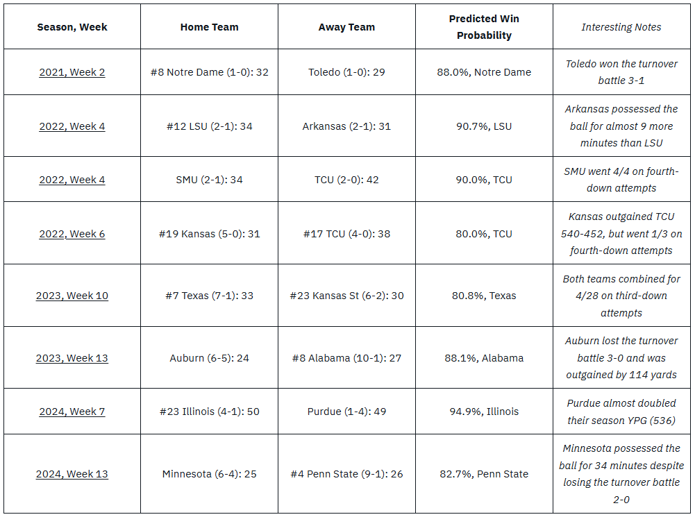
These results don’t necessarily indicate anything in the aggregate, as these games were close for a variety of reasons (one team playing up, another team playing down, turnovers, fourth downs, etc.), but it does suggest that these teams experienced at least some amount of good fortune. When evaluating an entire season (as opposed to just testing data), you can begin to evaluate if a team truly got lucky repeatedly and their record may suggest that they were better than in reality. For example, it is interesting that 2022 TCU is listed here twice, despite this dataset only containing 14 games from 2022 that fit the criteria.
Moving forward, this is something I plan to do at the end of each season — in essence, retraining the model on the season-end data and recalculating all game probabilities.
Conclusion
As previously mentioned, I plan to run both the base and the slimmed models throughout the 2025 season to determine which is actually more effective at predicting outcomes when working with completely unseen data. While these models are far from perfect, I’m extremely excited to observe their accuracies as the 2025 season plays out. Starting in Week 4 (September 20th), I plan to release short articles containing predictions ahead of each week’s slate of games, followed by recap articles that keep track of wins and losses, along with anything particularly notable.
This started off as taking something interesting I learned in school (data science and applied statistics) and applying it to my greatest passion, college football. A year and a half ago, I made a simple linear regression model comparing expected wins to actual wins based on team talent composites. In the time since then, I’ve dedicated free time in spurts to this burning interest of mine, culminating in these two logistic regression models. Over 50 hours have gone into the brainstorming, designing, developing, troubleshooting, redesigning and redeveloping, and finally, the documentation of these models. It has been a long road and I could not be more excited to see them in action throughout the upcoming season.
- I removed all FBS vs. FCS matchups because it is quite difficult to find comprehensive data on FCS schools, much less make it usable for analysis. ↩︎
- I’m planning on creating a model for neutral site games at some point in the future. This would be especially useful for predicting the College Football Playoff. ↩︎
- This is one of the most significant constraints of my model, and is touched on in a section below. ↩︎
- Surprisingly, things like completion percentage and yards per attempt aren’t included in the database cfbfastR pulls from (CFBD), or the developers of cfbfastR decided not to include these statistics in their functions. Either way, the necessary statistics to calculate these are included. ↩︎
- The actual math behind how stepwise regression works is beyond my understanding, but more information can be found here. ↩︎
- I considered using the same variables for continuity, but felt this would undermine the value in using a stepwise model in the first place. To reiterate, the first model is just to give me an idea of how accurate the stepwise model may be; it holds no real value moving forward. ↩︎
- Consider the MLB and NBA playoffs that utilize best-of series formats. Very, very rarely does the “lesser” team win, because these teams are given 5 to 7 games to prove themselves, eliminating much of the randomness that we see in a tournament like the NCAA’s March Madness. ↩︎
- For nail-biter games, it’s actually helpful that the model uses season-end data, as we’re able to objectively observe which games played out much closer than expected, based on each team’s overall quality. ↩︎
- It is frankly absurd that a turnover-on-downs isn’t considered a turnover in the box score — it’s literally in the name. ↩︎

Leave a comment