This post effectively serves as an addendum to the main article linked here, so it will be much more matter-of-fact. After all, that is basically what this model is — an add-on to the prior model to serve the ~20 games per year that are played on neutral sites (CFP included).
This model follows a similar format to the home/away model in that there is a base version and slimmed version. In this case, the slimmed version performs better than the base version. This is what I thought would happen in the home/away model, but given that the inverse is true, I decided to keep both versions for that model. For the sake of consistency, I’ll do the same here (though it likely isn’t going to do much good).1
Below are the accuracies for each version of the neutral site model:
| Base Model | 71.74% |
| Slimmed Model | 76.09% |
Methodology
I would argue this is where the real meat of this article is, as opposed to the prior article, where a lot of the interesting points concern constraints and findings. While I assumed that creating this neutral site model would be fairly straightforward, just filtering for neutral site games instead of solely home/away, I ran into an interesting problem.
The issue occurred to me during the design phase of the model. The home/away model uses predictors that are mapped to each team’s statistics, labeling these statistics “home_<statistic>” and “away_<statistic>“. I was fine with this because I see it as a means of accounting for home field advantage.
The home team wins more often than the away team, so when the model is being trained on this large dataset, the home team’s statistics would be weighed slightly higher in the model. Meaning, in a vacuum, if both “home_<statistic>” and “away_<statistic>” were equal, the home team would be slightly favored to win because that home-field advantage is essentially baked into the pie. In math terms, any given variable for the home team should have a higher coefficient (in terms of increasing the home team’s win probability) than the equivalent variable for the away team.
This structure presented a huge problem for the neutral site model. A number of the games in the training dataset included conference championships2, in which the better team is awarded the home designation. This opened the door for some amount of bias toward the home team to be built into the model, via the method described in the paragraph above.
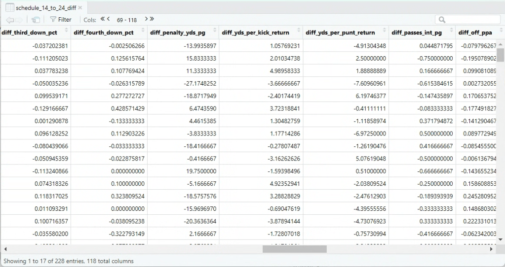
After some brainstorming and research, I came to the conclusion that I had to create what I’m colloquially calling a “differential data frame”. Essentially, I created columns in the data frame that represented the difference between the equivalent home and away statistics. Below is a screenshot of what this looked like:
This made it so the model could not bias toward home/away by combining the statistics for each into one column, so only one coefficient could be calculated for these statistics (as opposed to being systemically higher for the home/away version).
Besides this, the methodology was almost exactly the same. I used cfbfastR to scrape statistics for each team for a given season, scraped the schedule for that season, joined the statistics onto the schedule data frame, and trained the model.
One thing I improved upon from the home/away model was properly implementing the for loop to calculate accuracy across 1000 iterations of training/testing data splits. The goal is to calculate summary statistics about the distribution of accuracies. I go into significantly more detail in the prior article, but essentially, I forgot to include a step for retraining the model based on that iteration of the training/testing split. Below is what the for loop looked like in the code for the slimmed version of the neutral site model. I’ve bolded the code that fixed the issue:
For Loop
iterations = 1000

accuracy_results_1 = data.frame(Iteration = numeric(),
                                Train_Accuracy = numeric(),
                                Test_Accuracy = numeric())

for (i in 1:iterations) {

  # performing split
  data_split = initial_split(schedule_14_to_24_diff, prop = 0.8)
  model_training_loop = training(data_split)
  model_testing_loop = testing(data_split)

  # retraining model - this is where I messed up in the home/away model (forgot to include this part)
  slimmed_model_loop = glm(home_result ~
                             diff_avg_time_of_poss +
                             diff_fumble_pct +
                             diff_first_downs_pg +
                             diff_third_down_pct +
                             diff_def_success_rate +
                             diff_def_pts_per_opp +
                             diff_def_standard_downs_success_rate +
                             diff_offense_rating +
                             diff_defense_rating, data = model_training_loop, family = binomial)

  # making predictions and adding into data frames
  train_predictions_loop = model_training_loop %>%
    mutate(predicted_win_probability = predict(slimmed_model_loop, newdata=., type = "response"))

  train_predictions_loop = train_predictions_loop %>%
    mutate(predicted_win = ifelse(predicted_win_probability >= 0.5, 1, 0))

  test_predictions_loop = model_testing_loop %>%
    mutate(predicted_win_probability = predict(slimmed_model_loop, newdata=., type = "response"))

  test_predictions_loop = test_predictions_loop %>%
    mutate(predicted_win = ifelse(predicted_win_probability >= 0.5, 1, 0))

  # calculating accuracy
  train_accuracy = mean(train_predictions_loop$predicted_win == train_predictions_loop$home_result) # calculates % of times the two columns match
  test_accuracy = mean(test_predictions_loop$predicted_win == test_predictions_loop$home_result)

  # adding into results df
  accuracy_results_1 = rbind(accuracy_results_1, data.frame(Iteration = i,
                                                            Train_Accuracy = train_accuracy,
                                                            Test_Accuracy = test_accuracy))
}
Here are the full testing accuracy statistics, through 1000 iterations, for the base and slimmed versions of the model:
| Testing Data Accuracy | Base Model | Slimmed Model |
| Median | 71.74% | 76.09% |
| Standard Deviation | 6.24% | 5.77% |
| Interquartile Range | 67.39% – 76.09% | 73.91% – 80.43% |
| Range | 52.17% – 93.48% | 56.52% – 93.48% |
As previously mentioned, it was quite surprising to me that the slimmed version performed better than the base version, considering the inverse is true for the home/away model. I believe this is likely due to the relatively small sample size (228 games) compared to the ~2800 games in the home/away model.
Constraints
All of the constraints from the other model apply to this one, but one constraint specific to this model is the previously mentioned small sample size.
The home/away model is trained on all home/away regular season games from 2021 to 2024. This was intentional, as I did not want to include games from the COVID year, nor did I want to stray too far from what I consider to be the current era of college football. It was only 10 years ago that it seemed nobody had an answer for the spread — I wanted to ensure that games from another era were not included in the training data.
This proved to be an impossible principle to follow when gathering data for the neutral site model. Between 2021 and 2024, only 96 neutral site games were played (excluding the CFP, see footnotes).3 I subsequently decided to scrape all neutral site games from the CFP era (CFP games excluded), leaving me with 228 games of training data. While I consider this enough to build a somewhat robust model, it is only a fraction of the training data used in the home/away model. This is why the ranges of testing data accuracies shown above are so much wider.
Next Steps
Moving forward, I will be running this model alongside the home/away model in weekly predictions. Most weeks there will be 0 to 1 neutral site games, meaning it could do very well or very poorly throughout the remainder of the season due to simple randomness. Still, this model’s performance should be fun to track, particularly during the playoff.
- There is some inconsistency in how I refer to the base vs. slimmed versions. In the first article, I referred to them as two distinct models that achieve the same thing, whereas here, I’m calling them two versions of the same model. I feel referring to them as two versions of the same model makes more sense, but I don’t feel that editing the old 3,500+ word article to match this naming convention would be worth the return. Sorry for the confusion. ↩︎
- I thought about including CFP games, but given the structure of the data frame, this would have meant manually removing ~450 bowl games for ~30 CFP games over 10 years. If the model performs poorly, this will be something I’ll look to in the future to improve performance. ↩︎
- Oddly, 2024 had 13 more neutral site games than 2023. ↩︎

Leave a comment